Data profiling in Python

pandas-profiling Python package is a great tool to create HTML profiling reports. For a given dataset it computes the following statistics:

• Essentials: type, unique values, missing values
• Quantile statistics like minimum value, Q1, median, Q3, maximum, range, interquartile range
• Descriptive statistics like mean, mode, standard deviation, sum, median absolute deviation, coefficient of variation, kurtosis, skewness
• Most frequent values
• Histogram
• Correlations highlighting of highly correlated variables, Spearman and Pearson matrixes

Prerequisites

• Install Python and the Jupyter Notebook
  • On Linux
  • On Windows
• Install pandas-profiling module
  • GitHub repo: https://github.com/pandas-profiling/pandas-profiling
  • With Anaconda:

    conda install -c conda-forge pandas-profiling
    

Profiling data from a CSV file

Let’s see how to use pandas-profiling package on a dataset from the University of California, Irvine: Communities and Crime Data Set

Start Jupyter Notebook

jupyter notebook

Create a new notebook

Load pandas and pandas_profiling

import pandas as pd
import pandas_profiling

Load data into a DataFrame object and cast categorical numeric columns

df=pd.read_csv("./data/communities.csv" , sep=',', na_values=["?"])
# Some other useful read_csv parameters
# encoding='UTF-8'
# low_memory=False
# parse_dates=["date_column_name"]

# Change Pandas DataFrame column data type
# df["y"] = pd.to_numeric(df["y"])
# df["z"] = pd.to_datetime(df["z"]) 
df['state'] = df['state'].astype('category')
df['community'] = df['community'].astype('category')
df['fold'] = df['fold'].astype('category')

Display the data profiling report in a Jupyter notebook

pandas_profiling.ProfileReport(df)

Or export it in an HTML file

profile = pandas_profiling.ProfileReport(df)
profile.to_file(outputfile="./report.html")

Profiling data from SQL Server database

## From SQL to DataFrame Pandas
import pandas as pd
import pyodbc

sql_conn = pyodbc.connect('DRIVER={SQL Server Native Client 11.0}; \
                            SERVER=server_name; \
                            DATABASE=db_name; \
                            Trusted_Connection=yes') 
query = "SELECT [BusinessEntityID],[FirstName],[LastName],
                 [PostalCode],[City] FROM [Sales].[vSalesPerson]"
df = pd.read_sql(query, sql_conn)

pandas_profiling.ProfileReport(df)

With credentials replace pyodbc.connect instruction with the following

sql_conn = pyodbc.connect('DRIVER={SQL Server Native Client 11.0}; \
                            SERVER=server_name; \
                            DATABASE=db_name; \
                            uid=User; \
                            pwd=password') 

As alternative you could consider the pymssql module.

Other data profiling commands

df.head()

df.describe()

df.isnull().any()

df.isnull().sum()

null_columns=df.columns[df.isnull().any()]
df[null_columns].isnull().sum()

df.isnull().any().any()

df.info()

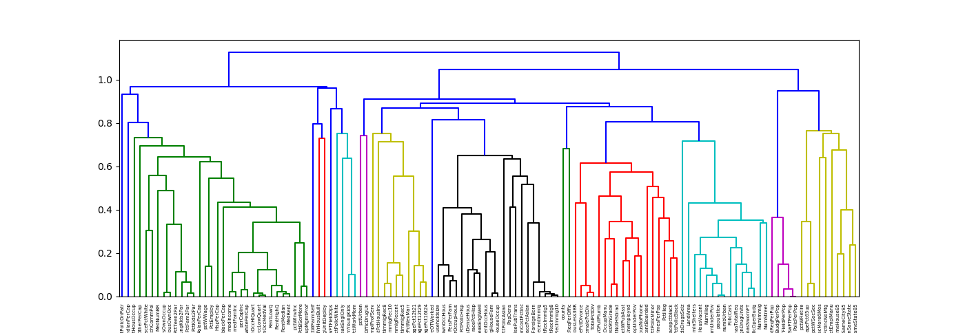
Plot a hierarchical clustering as a dendrogram.

%matplotlib notebook
import matplotlib.pyplot as plt
from scipy.cluster import hierarchy as hc

corr = 1 - df.corr() 
corr_condensed = hc.distance.squareform(corr) # convert to condensed
z = hc.linkage(corr_condensed, method='average')
dendrogram = hc.dendrogram(z, labels=corr.columns)

Principal Component Analysis (PCA) in Python (https://stackoverflow.com/a/50572561/9489744)

%matplotlib notebook
import numpy as np
import matplotlib.pyplot as plt
from sklearn import datasets
from sklearn.decomposition import PCA
import pandas as pd
from sklearn.preprocessing import StandardScaler

iris = datasets.load_iris()
X = iris.data
y = iris.target
X = iris.data
y = iris.target
#In general a good idea is to scale the data
scaler = StandardScaler()
scaler.fit(X)
X=scaler.transform(X)    

pca = PCA()
x_new = pca.fit_transform(X)

def myplot(score,coeff,labels=None):
    xs = score[:,0]
    ys = score[:,1]
    n = coeff.shape[0]
    scalex = 1.0/(xs.max() - xs.min())
    scaley = 1.0/(ys.max() - ys.min())
    plt.scatter(xs * scalex,ys * scaley, c = y)
    for i in range(n):
        plt.arrow(0, 0, coeff[i,0], coeff[i,1],color = 'r',alpha = 0.5)
        if labels is None:
            plt.text(coeff[i,0]* 1.15, coeff[i,1] * 1.15, "Var"+str(i+1), color = 'g', ha = 'center', va = 'center')
        else:
            plt.text(coeff[i,0]* 1.15, coeff[i,1] * 1.15, labels[i], color = 'g', ha = 'center', va = 'center')
plt.xlim(-1,1)
plt.ylim(-1,1)
plt.xlabel("PC{}".format(1))
plt.ylabel("PC{}".format(2))
plt.grid()

#Call the function. Use only the 2 PCs.
myplot(x_new[:,0:2],np.transpose(pca.components_[0:2, :]))
plt.show()